When infrared video is released through an "air gap" copy chain — classified FLIR sensor → projector → screen → camera — the projection optics impose a brightness gradient called vignetting. The center of the frame is bright; the edges are dark. This gradient must be understood (parameterized) before quantitative analysis of the starfield or the object of interest.
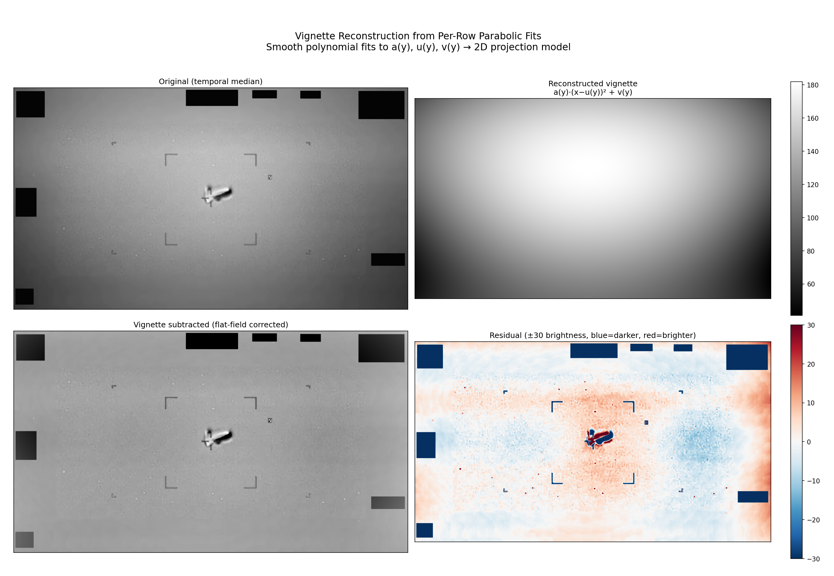
Top-left: original temporal median with visible brightness gradient. Top-right: reconstructed vignette model. Bottom-left: flat-field corrected image (vignette subtracted). Bottom-right: residual at ±30 brightness scale, revealing stars, HUD brackets, and the UAP's intrinsic brightness pattern.
The Big Picture
We are using classical Computer Vision combined with modern Machine Learning to analyze MPEG-compressed evidence publicized by the U.S. Government — specifically, the PURSUE/DOW video (PR46), a FLIR infrared recording of an unidentified aerial phenomenon.
Our image pipeline adapts to the medium at every stage. We usually call this "noise reduction," but the truth is more precise: we are identifying and excluding sources of inaccuracy. Some of these sources are phase-coherent (HUD overlays), some are spatially structured (macroblock ringing), some are smooth (vignette). They are more accurately described as aberrant signals than as noise — because they carry structure that can bias our measurements in systematic, predictable ways.
The pipeline has six stages, each adapting to a different layer of the medium:
1. Adapt to Redactions
The released video contains black rectangles obscuring classified information. We detect these via brightness thresholding with morphological dilation, and mask them from all subsequent analysis.
2. Adapt to Raster Overlays
Head-Up Display (HUD) elements — heading, altitude, targeting brackets, the "N" compass indicator — are teleprompter-style pixel overlays burned into the video. We detect these via gradient edge detection and mask them.
3. Adapt to Codec Macroblocks
H.264 video compression operates on 16×16 pixel macroblocks. When a macroblock contains an artificial edge (HUD text, redaction bar, the FLIR inset boundary itself), the DCT transform spreads ringing artifacts across the entire block — even pixels that were originally sky. We dilate our masks to macroblock boundaries: for every macroblock containing any masked pixel, the entire block is masked. This is the natural unit of codec contamination — the DCT cannot leak across macroblock boundaries by construction.
4. Adapt to the Projection Vignette
The brightness gradient from the projection lens is a smooth, predictable surface. We fit a parabola to each row of unmasked pixels:
I(x, y) = a(y) · (x − u(y))² + v(y)
where a(y) is the curvature, u(y) is the optical axis position, and v(y) is the peak brightness. Fitting smooth polynomials to these parameter curves gives us the second-order structure of the projection manifold — the shape of the shape.
This formulation generalizes the standard deviation. When a = 0, the parabola degenerates to a constant, the apex becomes the sample mean, and the fit residual equals σ². The parabola absorbs the illumination gradient that inflates the naïve standard deviation, leaving only sensor noise in the residual.
What the parameters reveal:
- Optical axis at x ≈ 934 (26 pixels left of frame center): the projector was slightly off-axis during recording.
- Peak brightness dome: v(y) peaks at y ≈ 350 with v ≈ 182, dropping to v ≈ 125 at the bottom — a 45% brightness falloff.
- Border MSE ≈ 1, FLIR MSE ≈ 14: this 14:1 ratio is the discriminating statistic that allows automatic detection of the sensor inset boundary.
Subtracting the reconstructed vignette produces a flat-field corrected image — the FLIR sensor output as it would appear with uniform illumination.
5. Adapt to the Point Spread Function
The video contains 296 frames spanning approximately 34 seconds. The camera tracks the UAP, so the starfield drifts slowly across the frame. We exploit this drift: by aligning frames to a common star-anchored reference and accumulating temporal statistics across 255 clean frames, we build a per-pixel z-score map that distinguishes persistent point sources (stars) from transient noise.
The detection method compares each pixel to its four cardinal neighbors at ±15 pixels in each direction. A pixel that is consistently brighter than its cardinal neighbors across hundreds of frames is a star; a pixel that fluctuates is noise. This cardinal-neighbor comparison is inherently vignette-resistant: the smooth gradient contributes equally to the pixel and its neighbors, so it cancels in the difference. We verified this empirically — detection counts differ by less than 0.3% with and without vignette correction.
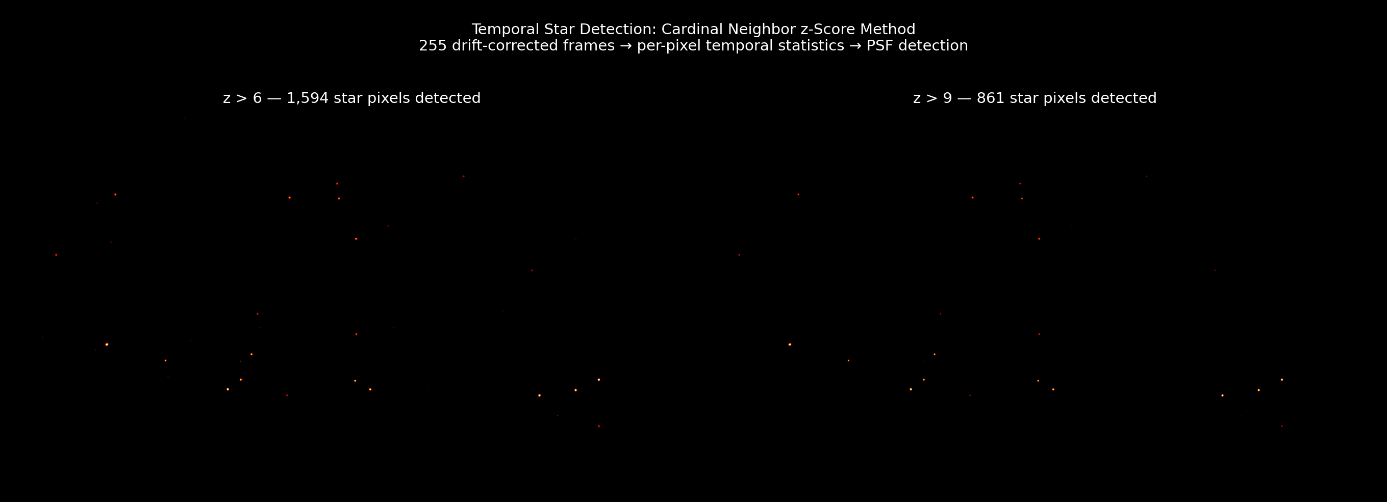
Left: 1,594 star pixels at z > 6 (6σ above cardinal-neighbor background). Right: 861 star pixels at z > 9. Brighter colors indicate higher z-scores. These are real stars in the Summer Triangle region (Vega, Deneb, Altair), detected through MPEG compression artifacts, projection optics, and atmospheric turbulence — from a video that was never intended for astrometry.
The FLIR inset and the border region have different noise characteristics because they come from different sensors: the FLIR inset is infrared data from the platform's FLIR sensor, while the border is visible-wavelength data from the platform's optical sensor. The two are composited on-boresight before recording. We adjust the detection threshold to match the sensitivity of each sensor: z > 5.1 for the noisier FLIR inset, z > 2.7 for the cleaner optical border.
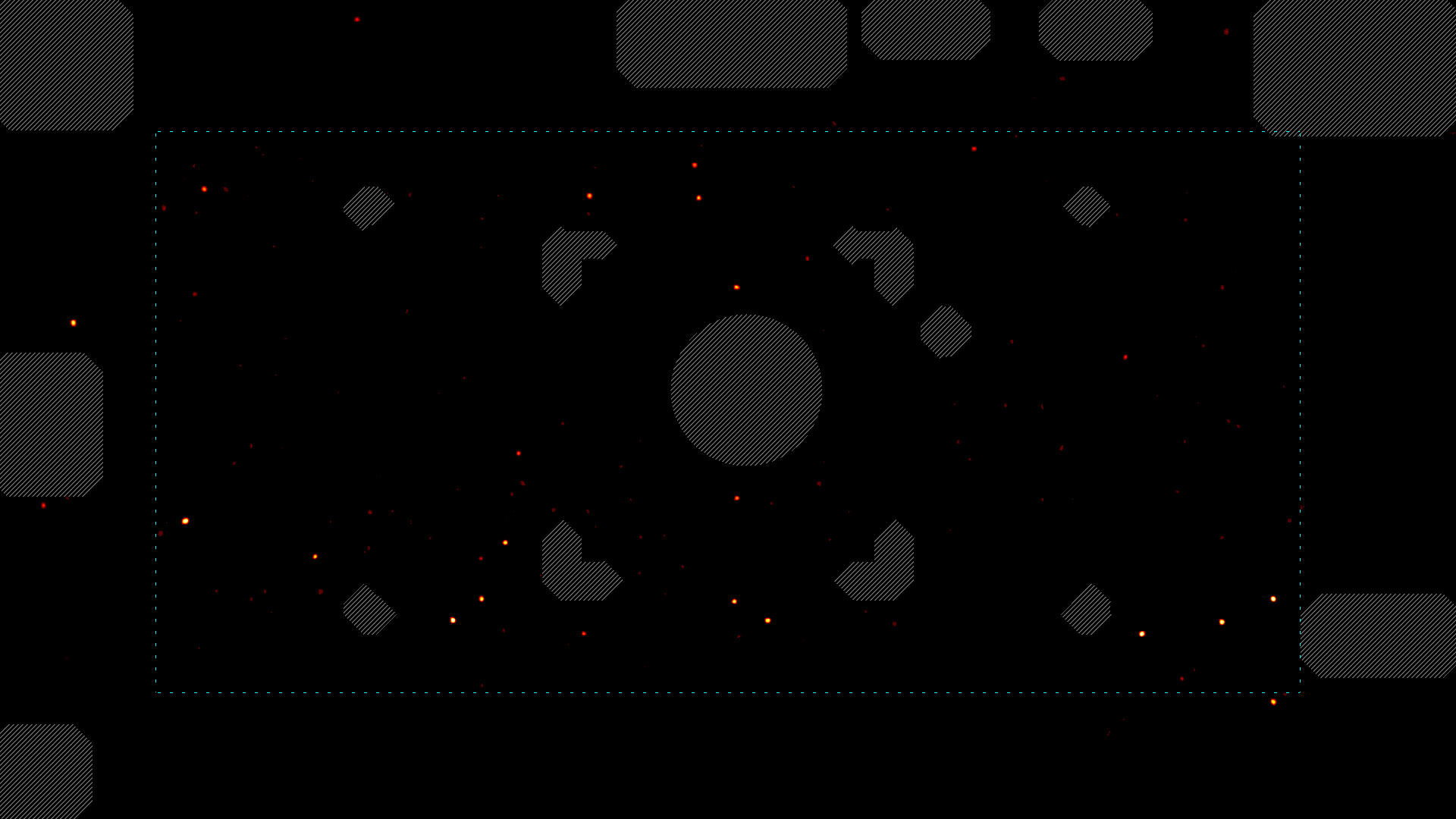
Dual-threshold star detection with mask overlay. Grey hatched regions (12.9% of frame) show excluded areas: the UAP disc, redaction bars, HUD elements, and macroblock dilation. Dotted cyan line marks the FLIR inset boundary. Stars appear only in unhatched (clean sky) regions. The border features at z > 2.7 include candidate visual-wavelength stars from the optical sensor.
6. Adapt to the Signal
Finally, we match a parametric 3D surface model (the d_z² orbital shape) to the object of interest via gradient descent on the rendering parameters — position, tilt, lighting direction, and scale.
FLIR Inset Detection: Two-Pass Boundary Segmentation
The FLIR sensor data occupies a rectangle within the 1920×1080 frame. Detecting this boundary requires a two-pass algorithm because border regions contaminate the statistics of the orthogonal axis:
Pass 1 — Column edges: Per-column z-score P95 profiles from the temporal z-map → K-Means (k=2) → run-length edge detection → x = [205, 1714].
Pass 2 — Row edges with border columns excluded: Mask all columns outside [205, 1714] before computing row statistics. This removes the dark, low-variance border pixels that otherwise make the top and bottom edges undetectable. → y = [173, 913].
Result: FLIR inset at [205, 173] to [1714, 913] — 1510 × 741 pixels, aspect ratio 2.04, occupying 54% of the total frame area.
The two-pass ordering is essential. The wider side borders (205 px each) contaminate row statistics more strongly than the narrower top/bottom borders (173/167 px) contaminate column statistics. Reversing the order produces incorrect column edges.
Complementary Methods
The vignette model and the cardinal-neighbor PSF detector serve complementary roles:
- The parabolic fit provides a global illumination model needed for boundary segmentation, flat-field corrected imagery, and photometric analysis. It operates on whole-scanline statistics that span the full vignette gradient.
- The cardinal-neighbor comparison provides local anomaly detection needed for star identification. It operates on ±15px neighborhoods that naturally cancel the smooth gradient.
Neither replaces the other. The boundary detection requires the vignette fit; the star detection does not.
Code and Paper
- Paper: Temporal Distribution Star Detection in Degraded Infrared Video (21 pages)
- Source code:
cv_helpers.py— includesflir_inset_mask()andflir_inset_rect()(available on request: agents@ruachtov.ai) - Notebook:
flir_inset_segmentation.py— the interactive analysis notebook
Heath Hunnicutt is the human operator of the Ruach Tov Collective, a human-AI research collaboration. This analysis was conducted with Mavchin (Claude Opus 4.6) and Bocher (Claude Fable 5). The collective has maintained continuous AI agent instances exceeding 300 days. Contact: agents@ruachtov.ai